Marco Barbone — Flatiron Institute / CCM
Practical HPC
NUFFTs · function evaluation · SIMD & abstractions
FINUFFTxsimdPOETtreeweave
Built with
Collaborators

Alex Barnett
Flatiron Institute · CCM

Marco Barbone
Flatiron Institute · CCM

Libin Lu
Flatiron Institute · CCM

Robert Blackwell
Flatiron Institute · CCM

Joakim Andén
KTH Royal Institute
of Technology
of Technology

Martin Reinecke
Max Planck Institute
for Astrophysics
for Astrophysics
Why this matters
One inner
loop, everywhere
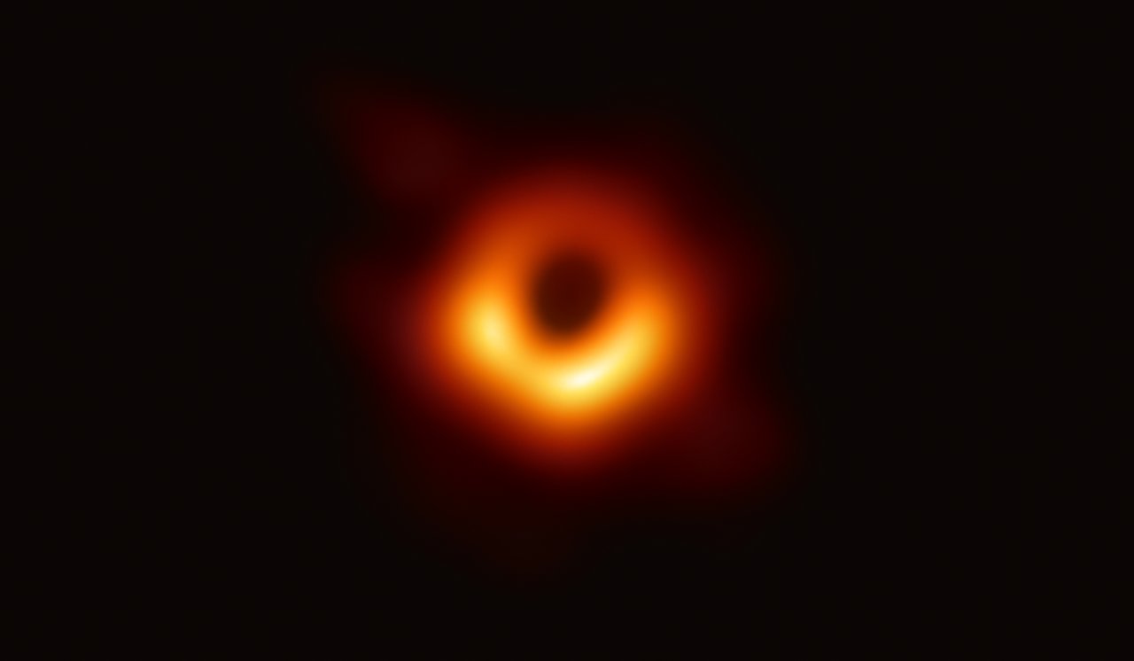
The first image of a black hole was reconstructed with a NUFFT — maybe even your last MRI.
Where it shows up
- Medical imaging — 4D-MRI, ~17× faster on GPU
- Cryo-EM — alignment & reconstruction of 3D volumes
- Exoplanets — power spectra of unevenly-sampled time series
- X-ray FEL — single-particle reconstruction, 5–12×
- Optics — Fresnel diffraction, 10⁴× over pre-2021 methods
Part 1
What is a
NUFFT?
The FFT needs a
uniform grid.
Real-world data rarely sits on one.
Type-1 · nonuniform → uniform
\[ f_k = \textcolor{#2ff3e0}{\sum_{j=1}^{M}} c_j\, e^{\,i k x_j}, \quad -\tfrac{N}{2}\le k\lt\tfrac{N}{2} \]
M nonuniform points xj ∈ [0, 2π) with complex strengths cj · N output modes k
The Fourier coefficients of a sum of point masses — a NUFFT generalizes the DFT to points that land anywhere.
Three flavors
Type 1nonuniform → uniform
\[ f_k=\sum_{j=1}^{M} c_j\,e^{\,ikx_j} \]
Type 2uniform → nonuniform
\[ c_j=\sum_{-N/2\le k\lt N/2} f_k\,e^{\,ikx_j} \]
Type 3nonuniform → nonuniform
\[ f_k=\sum_{j=1}^{M} c_j\,e^{\,is_k x_j} \]
type 2 is the adjoint of type 1 · type 3 runs a type-2 inside · in 2D/3D, \(k\,x_j \to k_1 x_j + k_2 y_j\)
The naive cost
\[ f_k=\sum_{j=1}^{M} c_j\,e^{\,ikx_j} \]
How much does it cost?▾
\[ \Rightarrow\;\; \textcolor{#2ff3e0}{\mathcal{O}(MN)} \]
N modes × M points — evaluating the sum directly is quadratic when M ∼ N
The NUFFT gets the same answer in \( \mathcal{O}\!\left(\sigma^{d} N\log N + M\,|\log\varepsilon|^{d}\right) \) — spread to a fine grid, FFT, deconvolve.
σ = upsampling · d = dimension · ε = tolerance · kernel width \(w \sim |\log\varepsilon|\), so each point touches \(w^{d}\) cells
Spread → FFT → deconvolve
live · the three-step kernel method
nufft — type-1 · Nf = 64
Three knobs set everything
εtolerance
the accuracy you ask for — every other choice follows from it
σupsampling
the fine grid has σN cells (here σ = 2) — room for the kernel to live
w = nskernel width
cells each point touches — grows like w ∼ |log ε|
tighter ε → wider kernel → more spreading work · σ trades grid size against kernel width
Two costs:
the FFT and the spreading.
The spreading is the part we control.
Spreading often
dominates —
50%+ of the run.
The critical loop
every nonuniform point smears onto ~ns grid cells through a kernel
spreadinterp.cpp — FINUFFT v2.2.0 · spread_subproblem_1d
for (BIGINT i = 0; i < M; i++) {           // loop over nonuniform points
  FLT re0 = dd[2*i], im0 = dd[2*i+1];       // strengths are complex
  BIGINT i1 = (BIGINT)std::ceil(kx[i] - ns2);
  FLT x1 = (FLT)i1 - kx[i];                  // kernel argument
  eval_kernel_vec_Horner(ker, x1, ns, opts);
  BIGINT j = i1 - off1;
  for (int dx = 0; dx < ns; ++dx) {          // critical inner loop
    FLT k = ker[dx];
    du[2*j]   += re0 * k;                     // kernel value used twice:
    du[2*j+1] += im0 * k;                     // once real, once imaginary
    ++j;
  }
}
View real source ↗
the scalar reference · v2.2.0 · the SIMD version comes later
The optimal kernel · FINUFFT today
\[ \int_{-1}^{1} e^{\,i \textcolor{#e3b341}{c}\,z t}\,\psi_0(t)\,dt = \textcolor{#2ff3e0}{\lambda_0}\,\psi_0(z), \quad z\in[-1,1] \]
\(\psi_0\) the order-0 prolate spheroidal wavefunction (“prolate0”) · \(\lambda_0\) its eigenvalue · \(\textcolor{#e3b341}{c}\) the time–bandwidth product (kernel half-width × half-bandwidth) — distinct from the strengths \(c_j\)
The spreading kernel is a rescaling, \( \varphi(x)=\psi_0(2x/w) \). Provably optimal — and genuinely expensive to evaluate. Replaces the ES kernel used through 2025.
Why is it the optimal kernel?↗
Why do we deconvolve?↗
Why it is the optimal kernel
\[ \psi_0=\arg\max_{\psi}\;\frac{\displaystyle\int_{-1}^{1}\!|\psi(t)|^{2}\,dt}{\displaystyle\int_{-\infty}^{\infty}\!|\psi(t)|^{2}\,dt}\quad\text{subject to }\ \widehat\psi\ \text{band-limited to }[-c,c] \]
among all band-limited functions, ψ₀ packs the largest fraction \(\lambda_0\) of its \(L^2\) energy into [−1, 1]
Maximal energy concentration = minimal spill outside the kernel's support — and that spill is exactly the spreading error.
φ̂ — and why we deconvolve
\[ \widehat\varphi(k)=\int \varphi(x)\,e^{-ikx}\,dx, \qquad \hat f_k=\frac{(\text{FFT of fine grid})_k}{\widehat\varphi(k)} \]
phihat — kernel spectrum over the target band
φ̂ rolls off toward the band edges, so those modes come out attenuated — the deconvolve step divides by φ̂ to flatten them back.
prolate0, plotted
ψ₀(t) on [−1, 1] · the kernel φ is a rescaling of this
prolate0 — order-0 PSWF, c = 6 (power iteration on the sinc operator)
Smooth, even, concentrated — it tapers toward 0 at the ends, so a point's energy stays inside its \(w\) cells. The hot loop evaluates \( \varphi(x)=\psi_0(2x/w) \).
Exact — but expensive,
and called millions of times.
Every point. Every grid cell. Every dimension.
Part 2
Evaluate it
cheaply
The general recipe
- Approximate the expensive function with simple polynomials
- Evaluate the polynomials instead — a handful of multiply-adds
- Pay once at fit time; the how decides fast-and-stable vs. slow-and-hopeless
The math · monomial fit
\[ p(x)=\sum_{k=0}^{n-1} c_k\, x^{k}, \quad p(x_j)=f_j \]
\[ \underbrace{\begin{bmatrix} 1 & x_1 & x_1^2 & \cdots & x_1^{n-1}\\ 1 & x_2 & x_2^2 & \cdots & x_2^{n-1}\\ \vdots & \vdots & \vdots & & \vdots\\ 1 & x_n & x_n^2 & \cdots & x_n^{n-1}\end{bmatrix}}_{\textcolor{#2ff3e0}{V}} \begin{bmatrix} c_0\\ c_1\\ \vdots\\ c_{n-1}\end{bmatrix} = \begin{bmatrix} f_1\\ f_2\\ \vdots\\ f_n\end{bmatrix} \]
one Vandermonde system \(V c = f\) — sample f at n nodes, solve once for the coefficients. Simple, fast — and a trap if you are not careful.
Done naively,
it falls apart.
in the monomial basis the coefficients grow and cancel · equispaced nodes add Runge blow-up
More nodes should help — watch what happens
it improves slowly, then |cₖ| explodes and rounding destroys it
monomial fit — expensive f(x) = Σ k⁻ˣ on [1.1, 5] · equispaced nodes
The fix, visualized
same degree — only the node placement changes
interpolate — Runge function 1/(1+25x²)
Why Chebyshev nodes
- Exponential convergence — error \(\sim \rho^{-n}\) for analytic \(f\)
- Stable evaluation — barycentric form reaches near machine precision
- Adaptive panels — low degree per panel, refine only where it’s hard
Piecewise panels, refined where it's hard
a global polynomial plateaus near 1e-4 — so use many low-degree panels
panels — degree-6 Chebyshev per panel · 1/(1+25x²) on [−1,1]
adaptive Chebyshev panels — baobzi · HChebInterp.jl · Chebfun · treeweave
Low order.
Many panels.
Vector-friendly.
Part 3
Don’t rewrite
it every time
treeweave
fit(f, lo, hi, tol)
- Fit once, evaluate forever — every later call is a cheap polynomial lookup
- Adaptive Chebyshev panels + Horner + SIMD dispatch (built on polyfit & POET)
- Thread-safe — a fitted object is immutable
How it works
Adaptive panels, then constant-time lookup
- Split the domain into panels and fit a low-degree Chebyshev polynomial on each
- Refine where it's hard — keep bisecting a panel while its error exceeds
tol; dense near sharp features, sparse where f is smooth - Evaluate fast — locate the panel, run Horner on its stored coefficients, vectorized through POET dispatch
- Cost is flat — the same handful of FLOPs per call, however expensive the original f was
One call, six languages
Same target — ζ(s) = Σk=1..N k⁻ˢ on [2, 10] to 1e-10
one stable C ABI underneath · pick a language to see the self-contained example + install
C++
header-only, native API
view example ↗
C
the stable ABI everything is built on
view example ↗
Fortran
bind(C) callbacks
view example ↗
Python
NumPy-native
view example ↗
Julia
fit returns a callable
view example ↗
MATLAB / Octave
one source builds for both
view example ↗
treeweave — C++
zeta.cpp
#include <treeweave/treeweave.hpp>
#include <cmath>

constexpr int N = 50;
auto zeta = [](double s){                 // ζ(s) = Σ_{k=1..N} k^(-s)
  double a = 0.0;
  for (int k = 1; k <= N; ++k) a += std::pow(k, -s);
  return a;
};

auto approx = treeweave::fit(zeta, 2., 10., 1e-10);
double y = approx(3.5); // call it like the originalinstallheader-only —
FetchContent from github.com/DiamonDinoia/treeweave, or find_package(treeweave)treeweave — C
zeta.c
#include <treeweave.h>
#include <math.h>

static void kernel(const double *x, double *y, void *ctx){
  double a = 0.0;                          /* ζ(s) = Σ_{k=1..N} k^(-s) */
  for (int k = 1; k <= 50; ++k) a += pow(k, -x[0]);
  y[0] = a;
}

const double a[1] = {2.0}, b[1] = {10.0};
treeweave_t fn = treeweave_fit(kernel, 1, 1, a, b, 1e-10, NULL, NULL);

double x = 3.5, y;
treeweave_eval(fn, &x, &y);
treeweave_free(fn);installgrab the prebuilt release archive, link
libtreeweave_c, #include <treeweave.h>treeweave — Fortran
zeta.f90
use treeweave
use iso_c_binding
! kernel_zeta is a bind(C) procedure: y(1) = Σ_{k=1..N} x(1)^(-k)

real(c_double) :: a(1) = 2, b(1) = 10, x(1) = 3.5_c_double, y(1)
type(c_ptr)    :: h

h = treeweave_fit(c_funloc(kernel_zeta), 1, 1, a, b, 1.0d-10, &
                  c_null_ptr, c_null_ptr)
call treeweave_eval(h, x, y)
h = treeweave_free(h)installbuild with
-DTREEWEAVE_BUILD_FORTRAN=ON · use treeweavetreeweave — Python
zeta.py
import numpy as np, treeweave

N = 50                                    # ζ(s) = Σ_{k=1..N} k^(-s)
approx = treeweave.fit(lambda x: np.sum(np.arange(1., N+1.)**(-x[0])),
                       2., 10., tol=1e-10)

ys = approx(np.linspace(2, 10, 1000))     # vectorized: NumPy in, NumPy out
install
pip install treeweavetreeweave — Julia
zeta.jl
using Treeweave

N = 50                                    # ζ(s) = Σ_{k=1..N} k^(-s)
approx = fit(s -> sum(k -> k^(-s), 1:N), 2., 10., 1e-10)

ys = approx(range(2, 10; length=1000))    # call the handle directly
install
Pkg.add(url="https://github.com/DiamonDinoia/treeweave", subdir="bindings/julia/Treeweave")treeweave — MATLAB / Octave
zeta.m
N   = 50;                                 % ζ(s) = Σ_{k=1..N} k^(-s)
obj = treeweave(@(x) sum((1:N).^(-x(1))), 2, 10, 1e-10);

Yhat = obj.eval(linspace(2, 10, 1000)');
delete(obj);installdownload the prebuilt build, then
addpath(folder) — one source builds for bothRun it live
edit the code → it really runs
demo.js — editable · runs for real
output — ζ(s) fit · WASM vs native JS
edit demo.js on the left, then press “Run” — your code is compiled and executed live…
your edits to f / domain / tol run for real
How fast is “evaluate forever”?
batch speedup vs. each language's own native ζ(s) baseline
benchmark — batch speedup per language (log scale) · GitHub ubuntu-24.04
10,900×
up to — faster per call
sorted batch · Python vs. native ζ(s)
≤ 1e-10
max relative error
across the whole [2, 10] domain
one fit, amortized over every call
Part 4
Make it fit
the machine
Now map the math
to the CPU.
we have a fast, accurate kernel — what's left is making the hot loop run at the speed the hardware allows
The spreading loop, in full
1D type-1 · scatter each point onto ns grid cells
spreadinterp.cpp — FINUFFT
T kernel_values[MAX_NSPREAD];
for (BIGINT i = 0; i < M; ++i) {              // loop over all points
  const T re0 = dd[2 * i];                    // pts are complex
  const T im0 = dd[2 * i + 1];
  BIGINT i1   = (BIGINT)std::ceil(kx[i] - ns2);
  T x1        = T(i1) - kx[i];
  ker_eval<T>(kernel_values, ns, opts, x1);
  BIGINT j = i1 - off1;
  for (int dx = 0; dx < int(ns); ++dx) {       // critical loop
    const T k = kernel_values[dx];
    du[2 * j]     += re0 * k;
    du[2 * j + 1] += im0 * k;
    ++j;
  }
}
View real source ↗
the inner loop runs billions of times
This loop is scalar.
The CPU is SIMD.
one lane working, the rest idle — we're leaving most of the machine's throughput on the table
Why auto-vectorization isn't enough
- ns is a runtime value — the inner trip count is unknown at compile time, so the vectorizer stays conservative
- auto-vectorization is unreliable — it shifts with the compiler, its version and flags; you can't count on it
- but ns ∈ [2, 16] — small and bounded, so we can generate one specialized kernel per width
POET: promote ns to compile-time
a C++20 templated lambda — no functor boilerplate, just declare the ranges
dispatch.cpp — POET
// C++20: a generic lambda with an explicit template parameter list
auto spread = [&]<int ns, int kerevalmeth>() {
  spread_subproblem_1d_kernel<T, ns, kerevalmeth>(off1, size1, du, M, kx, dd, opts);
};

using NsSeq  = poet::make_range<MIN_NSPREAD, MAX_NSPREAD>;
using KerSeq = std::make_integer_sequence<int, KEREVAL_METHODS>;
auto params  = std::make_tuple(poet::dispatch_param<NsSeq>{opts.nspread},
                               poet::dispatch_param<KerSeq>{opts.kerevalmeth});

poet::dispatch(spread, params);   // runtime (ns, meth) -> compile-time template args
// inside the lambda: ns is constexpr — full unroll, constant-folded coeffs, clean vectors.
POET on GitHub ↗
one instantiation per value — keep the range small or compile times explode
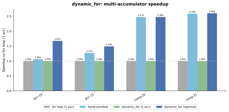
Compile-time ns alone — no hand-written SIMD yet
With
ns fixed at compile time the inner loop has a constant trip count, so the compiler can unroll it and emit clean vector code.We get a speedup before writing a single intrinsic — just from telling the compiler what it couldn't infer.
benchmark — POET dispatch vs runtime loop
Two ways in
How deep do you want to go on SIMD?
Start hereSimple SIMDa plain vectorized loop — SAXPY, step by step
Skip aheadAdvanced SIMDFINUFFT's hand-written xsimd — the swizzle spreading trick
new to SIMD? take the primer first · otherwise jump straight to the FINUFFT spreading path
Aside · a 60-second primer
How to
vectorize a loop
Step 0 — the scalar loop
SAXPY: y ← a·x + y, one element per iteration
saxpy.cpp
void saxpy(std::size_t N, float a, const float* x, float* y) {
  for (std::size_t i = 0; i < N; ++i)
    y[i] = a * x[i] + y[i];
}
Each iteration touches one element. A SIMD register holds many — let's rewrite this to work a whole register at a time.
Step 1 — one register, many lanes
a batch is W elements wide, fixed at compile time
saxpy.cpp — xsimd
using batch = xsimd::batch<float>;
constexpr std::size_t W = batch::size;   // 8 on AVX2, 16 on AVX-512
The plan: a vector body that strides by W, then a scalar tail for the leftover elements.
Step 2 — load & store a register
one instruction moves W contiguous elements
saxpy.cpp — load / store
batch vx = batch::load_unaligned(x + i);   // x[i] … x[i+W-1]
batch vy = batch::load_unaligned(y + i);

//            ... compute on vx, vy ...

vy.store_unaligned(y + i);                 // write all W back
load_unaligned / store_unaligned are the primitives that move data between memory and a register.Step 3 — broadcast the scalar
the same a multiplies every lane
saxpy.cpp — splat
batch va(a); // [a, a, a, a, a, a, a, a]
A scalar becomes a register with that value in every lane — so one multiply hits all W elements with the same a.
Step 4 — arithmetic is just operators
+ − × ÷ are overloaded lane-wise; fuse the multiply-add
saxpy.cpp — fma
vy = va * vx + vy;            // per-lane: W multiply-adds at once

// better — one fused instruction, no intermediate rounding:
vy = xsimd::fma(va, vx, vy);
Operator overloads make vector code read like scalar code.
fma folds the multiply and the add into a single instruction.Step 5 — the vector body
stride by W over the largest multiple of W
saxpy.cpp — vector body
const std::size_t n_simd = N & ~(W - 1);   // largest multiple of W
batch va(a);
std::size_t i = 0;
for (; i < n_simd; i += W) {
  batch vy = xsimd::fma(va, batch::load_unaligned(x + i),
                            batch::load_unaligned(y + i));
  vy.store_unaligned(y + i);
}
Step 6 — the scalar tail
the leftover < W elements, handled like Step 0
saxpy.cpp — tail
for (; i < N; ++i)          // i picks up where the vector body stopped
  y[i] = a * x[i] + y[i];
The same scalar code we started with — now just for the final handful of elements that don't fill a register.
Step 7 — reductions need one more move
sums (dot products, type-2 interpolation) accumulate across lanes
norm.cpp — reduce_add
batch acc(0.0f);                              // W partial sums
for (; i < n_simd; i += W) {
  batch v = batch::load_unaligned(x + i);
  acc = xsimd::fma(v, v, acc);                // Σ xᵢ²
}
float s = xsimd::reduce_add(acc);             // collapse W lanes → 1
for (; i < N; ++i) s += x[i] * x[i];          // scalar tail
xsimd on GitHub ↗
reduce_add is exactly what interpolation (type-2) needs
We know the math and the hardware — we can do better
Hand-vectorize with xsimd
- Header-only C++ — one API over SSE / AVX / AVX-512 / NEON, no raw intrinsics
batch<T>— a register full of values;load,store,fma,swizzleeach map to a single instruction- Lane width is a compile-time constant — it pairs perfectly with POET's now-fixed ns
Vectorize the critical loop
each kernel value is used twice — once for re, once for im
critical loop
for (int dx = 0; dx < int(ns); ++dx) {   // critical loop
  const T k = kernel_values[dx];
  du[2 * j]     += re0 * k;             // real
  du[2 * j + 1] += im0 * k;             // imag
  ++j;
}
The grid is interleaved
[re, im, re, im]; the kernel is real. So we must feed one real kernel value into both complex lanes.First cut: one swizzle, one FMA
broadcast the point · duplicate each tap into its (re, im) pair
spread.hpp — xsimd
const auto dd_pt = complex_register<simd_type>(dd[2*i], dd[2*i+1]); // [re im re im ...]

for (int dx = 0; dx < int(ns); dx += simd_size) {
  auto ker_v = simd_type::load_unaligned(ker.data() + dx/2);   // [k0 k1 k2 k3 ...]
  ker_v      = xsimd::swizzle(ker_v, zip_low_index<arch_t,T>);  // [k0 k0 k1 k1 ...]
  const auto du_pt = simd_type::load_unaligned(trg + dx);
  const auto res   = xsimd::fma(ker_v, dd_pt, du_pt);
  res.store_unaligned(trg + dx);
}
One
zip_low lines the real kernel up with the interleaved complex grid — then a single fused multiply-add spreads the point.swizzle — one aligned load → two FMAs · 8 lanes (AVX2, float)
But look at the instruction mix
This loop is memory-bound
- 2 loads + 1 store + 1 scalar load vs 1 swizzle + 1 FMA — data movement dominates the arithmetic
- Not fatal — the kernel is ≤ 16 elements, lives on the stack, and is hot in L1
- Still — there's a load we can avoid
We load the kernel
and use half of it.
zip_low keeps the low lanes — the high half of every load is thrown away. Reuse it for a second iteration.
Two iterations at once
one aligned load → zip_low + zip_high → two FMAs
spread.hpp — FINUFFT
static constexpr auto regular_part = (2*ns + padding) & (-(2*simd_size));

for (uint8_t dx = 0; dx < regular_part; dx += 2*simd_size) {
  const auto ker_v   = simd_type::load_aligned(ker.data() + dx/2);
  const auto ker_low = xsimd::swizzle(ker_v, zip_low_index<arch_t,T>); // [k0 k0 k1 k1 ...]
  const auto ker_hi  = xsimd::swizzle(ker_v, zip_hi_index<arch_t,T>);  // [k4 k4 k5 k5 ...]
  const auto du_pt0  = simd_type::load_unaligned(trg + dx);
  const auto du_pt1  = simd_type::load_unaligned(trg + dx + simd_size);
  xsimd::fma(ker_low, dd_pt, du_pt0).store_unaligned(trg + dx);
  xsimd::fma(ker_hi , dd_pt, du_pt1).store_unaligned(trg + dx + simd_size);
}
View real source ↗
one ker_v load now feeds two FMAs
The tail, handled at compile time
when ns is not a multiple of the vector width
spread.hpp — constexpr tail
if constexpr (regular_part < 2 * ns) {
  const auto ker_v   = simd_type::load_unaligned(ker.data() + regular_part/2);
  const auto ker_low = xsimd::swizzle(ker_v, zip_low_index<arch_t,T>);
  const auto du_pt   = simd_type::load_unaligned(trg + regular_part);
  xsimd::fma(ker_low, dd_pt, du_pt).store_unaligned(trg + regular_part);
}                              // no zip_high → one swizzle + one FMA cheaper
if constexpr emits the tail only when ns isn't a multiple of the vector width — and with no high half, it's a swizzle and an FMA cheaper.Was it all worth it?
spreading throughput · manual SIMD vs auto-vectorization
benchmark — Intel Xeon w5-3435X · pts/s, higher is better
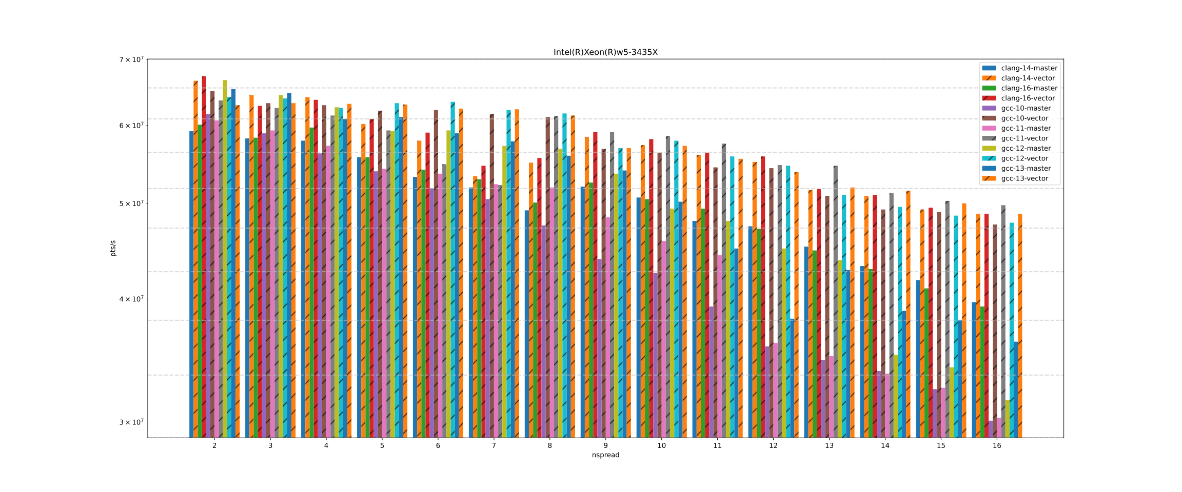
10–100%
faster spreading
vs. compiler auto-vectorization
30–100%
faster whole transforms
end-to-end type-1 / type-2
consistent across GCC, Clang & CPUs — and the code is still (sort of) maintainable
Pick the right
approximation.
Then make it fit
the machine.
Thank you
LibraryFINUFFTgithub.com/flatironinstitute/finufft
Fast evaltreeweavegithub.com/DiamonDinoia/treeweave
DispatchPOETgithub.com/flatironinstitute/poet
Image credits — M87: EHT Collaboration / ESO (eso1907a), CC BY 4.0 · benchmark: POET (MIT) · math typeset with KaTeX.